Plotting a Pole Figure
Important
Read first: Visualizing a Tessellation.
A pole figure can be generated using the Visualization Module (-V), by switching to pole figure space, using -space pf. Pole figures can be generated from one or several inputs, among those of the Visualization Module (-V), such as the orientations of a tessellation cells, an orientation file and/or a direction file, making it possible to produce advanced figures.
Note
Inverse pole figures can be plotted just as pole figures, using -space ipf instead of -space pf. Inverse pole figures are used in Plotting Orientation Trajectories.
Visualization in pole figure space works in the same way as visualization in standard, real space: the entity properties can be specified using the -data* options, the entities to show can be specified using the -show* options, etc. A difference is that the list of entities reduces to cell if the input is a tessellation, and <input> (or the default point) if the input is a custom input (orientations or directions).
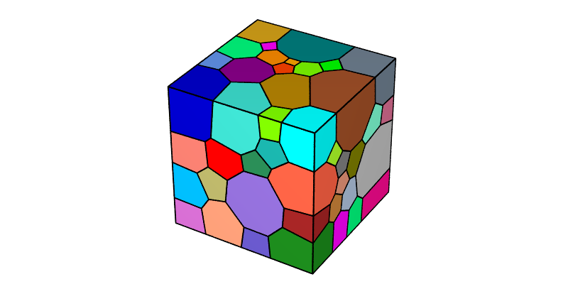
In the following, and unless mentionned otherwise, a simple tessellation is used:
# $ neper -T -n 100 -morpho gg -oricrysym cubic -o n100
The tessellation can be visualized as follows:
$ neper -V n100.tess -imagesize 800:400 -print img1
To reproduce exactly the images below, add the following line to your $HOME/.neperrc file (or to a local configuration file to be loaded with --rcfile):
neper -V -imagesize 500:500
Generalities
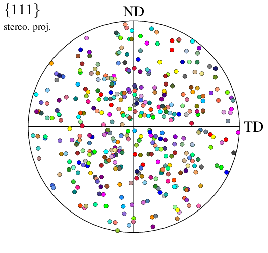
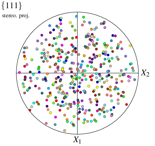
The tessellation orientations can be visualized using -space pf:
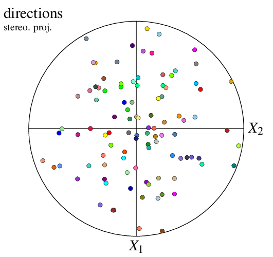
$ neper -V n100.tess -space pf -print img2
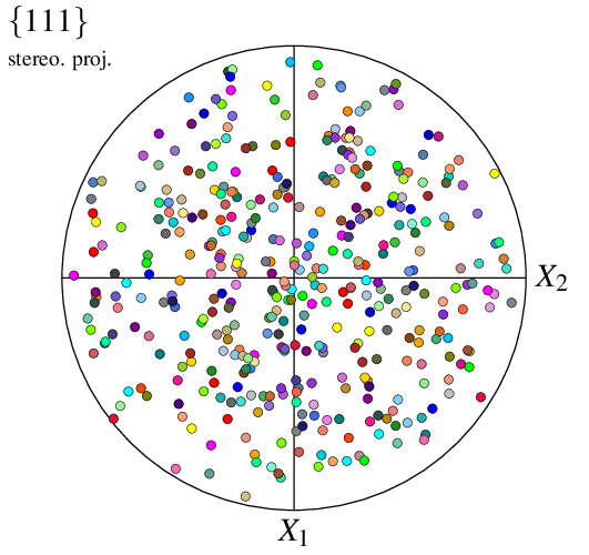
This generates a PNG image named img2.png. By default, a pole figure is plotted from the (four) {111} poles, using a stereographic projection in the 1–2 reference plane, and all cell orientations/poles are represented using symbols. Orientations are colored from their (cell) ids, so that colors match between visualizations in real space an pole figure space (the two images above).
Note
Even if only orientations/poles are represented in pole figure space, cell is used to represent a cell orientation, which makes it possible to use the same options, -showcell, -datacellcol, etc. in all spaces.
For pole figures, it is also possible to write the output file at a vectorial PDF format:
$ neper -V n100.tess -space pf -imageformat pdf -print img2
Note
The PDF format, as a vectorial format, provides an optimal quality/weight ratio and should be used when possible (for example, in LaTeX documents).
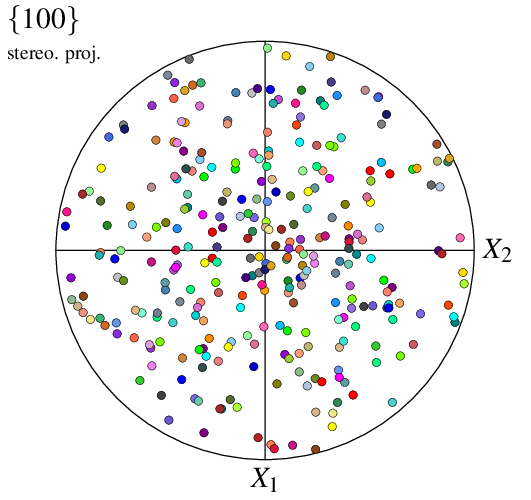
The pole family can be modified using -pfpole:
$ neper -V n100.tess -space pf -pfpole 1:0:0 -print img3
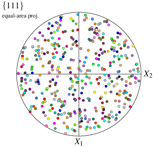
The projection type can be modified using -pfprojection:
$ neper -V n100.tess -space pf -pfprojection equal-area -print img4
The sample directions can be modified using -pfdir, so as the actual axis labels, using -datacsyslabel:
$ neper -V n100.tess -space pf -pfdir y:z -datacsyslabel RD:TD:ND -print img5
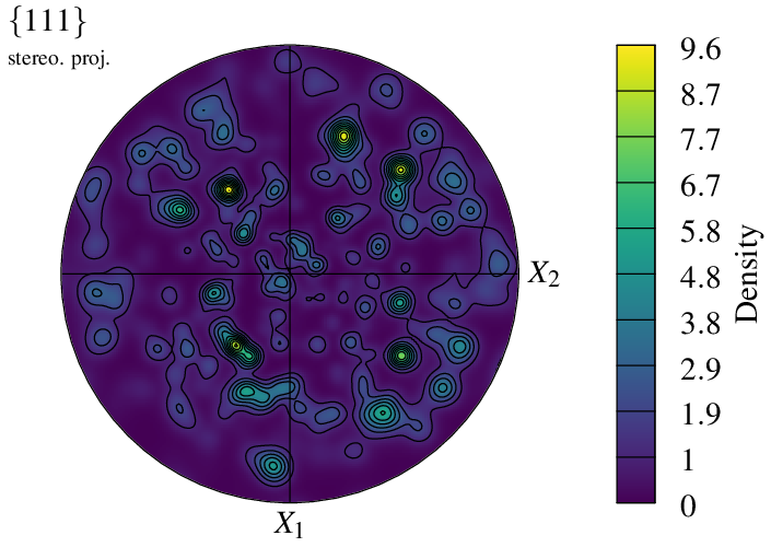
The representation mode can be changed into density:
$ neper -V n100.tess -space pf -pfmode density -print img6
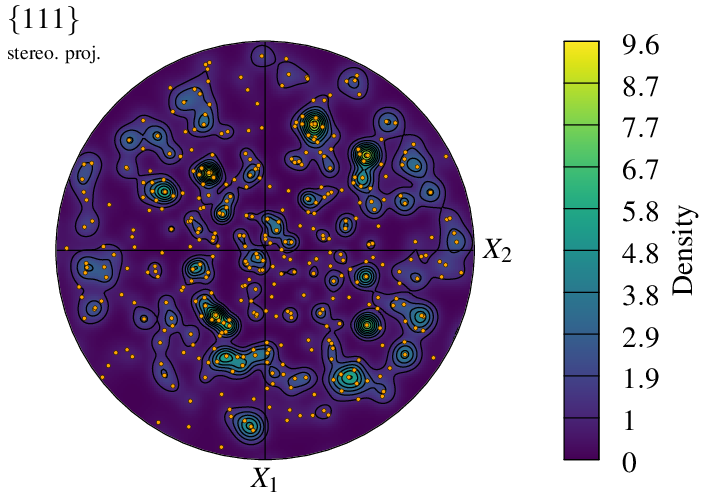
It is even possible to superimpose the symbol and density representation modes:
$ neper -V n100.tess -space pf        \
        -pfmode density,symbol        \
        -datacellcol orange           \
        -datacellrad 0.01             \
        -print img7
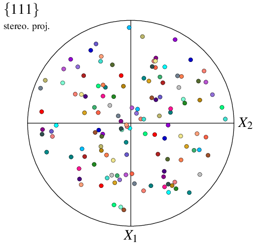
The visualization can be reduced to a selection of cells using -showcell (as in real space). For instance, to show only the cells larger than the average:
$ neper -V n100.tess -space pf -showcell "vol>0.01" -print img8
Finally, it is possible to change the character font from the default TimesRoman to the LaTeX-style ComputerModern:
$ neper -V n100.tess -space pf -pffont ComputerModern -print img9

Configuring a Symbol Plot
For a tessellation, the way data are represented can be specified using options -datacell*. The properties include the color (options -datacellcol and -datacellcolscheme),
transparency (option -datacelltrs), radius (or size) (option -datacellrad) and symbol (option -datacellsymbol).
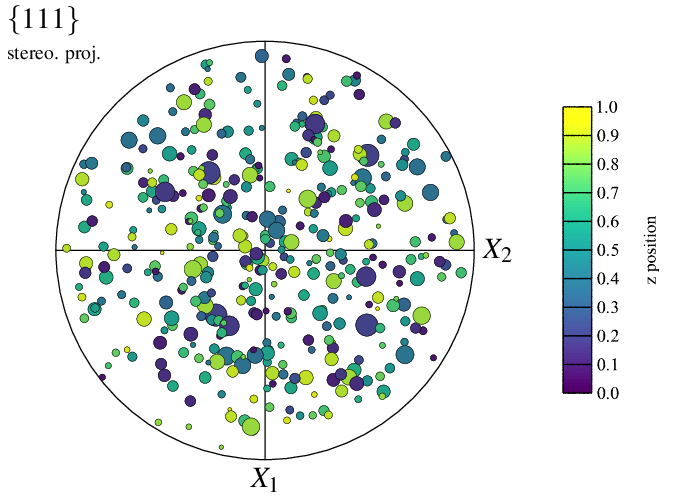
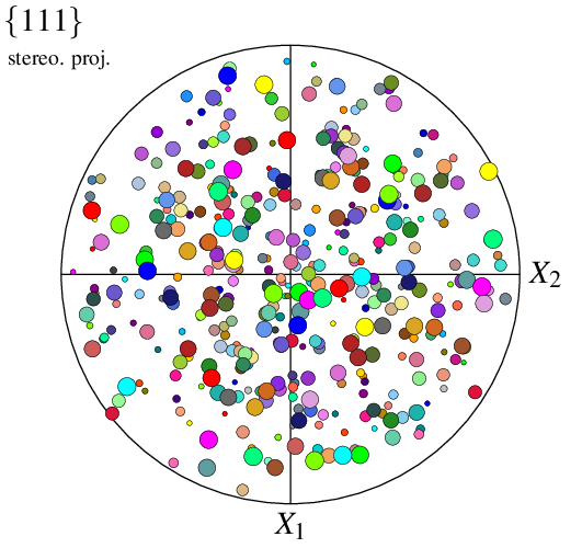
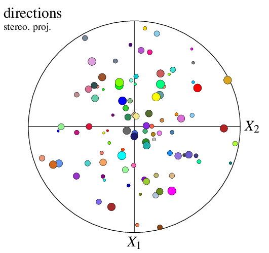
The size of the poles can, for instance, be set to be proportional to the corresponding cell sizes, and their colors a function of the z cell positions:
$ neper -V n100.tess -space pf              \
        -datacellrad real:0.1*diameq        \
        -datacellcol z                      \
        -datacellscale "0.0:1.0"            \
        -datacellscaletitle "z position"    \
        -print img10
$ convert +append img10.png img10-scale3.png -alpha off img10.png
This originally produces a PNG file named img10.png for the map and a PNG file named img10-scale3.png for the scale bar, which is pasted to img10.png thanks to convert.
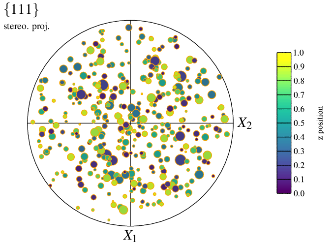
The apparence of the symbol “edges” can also be specified, using options -datacelledgerad and -datacelledgecol. For example:
$ neper -V n100.tess -space pf                  \
  -datacellrad real:0.1*diameq                  \
  -datacellcol z                                \
  -datacellscale "0.0:1.0"                      \
  -datacellscaletitle "z position"              \
  -datacelledgerad 0.02                         \
  -datacelledgecol orange                       \
  -print img11
$ convert +append img11.png img11-scale3.png -alpha off img11.png
The type of symbols can be specified using -datacellsymbol. For example, to use squares:
$ neper -V n100.tess -space pf                  \
  -datacellrad real:0.1*diameq                  \
  -datacellsymbol "square"                      \
  -print img12
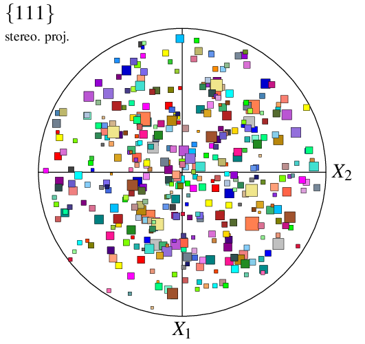
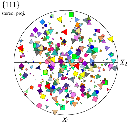
When only the type of symbol is provided to -datacellsymbol, the radius is taken from option -datacellrad (either the provided value or the default value). Alternatively, values can be provided in -datacellsymbol itself, as well as an angle; different symbols can even be specified for the different cells, using a Data File (n100-symbols), to produce a fully customized plot:
$ neper -V n100.tess -space pf                 \
  -datacellsymbol "file(n100-symbols)"         \
  -print img13
Configuring a Density Field Plot
A tessellation with typical rolling orientations is used in the following: n200-psc.tess.
The (default) symbol plot can be turned into a density field plot using -pfmode density.
$ neper -V n200-psc.tess -space pf            \
           -pfmode density                    \
           -print img14
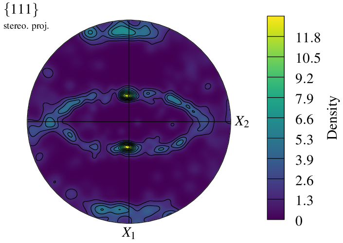
A density plot is plotted with a color field and contour lines that correspond to the scale ticks.
The scale extent and ticks (and so the values of the contour lines) can be modified using -datacellscale:
$ neper -V n200-psc.tess -space pf            \
           -pfmode density                    \
           -datacellscale 0:2:4:6:8:10:12     \
           -print img15
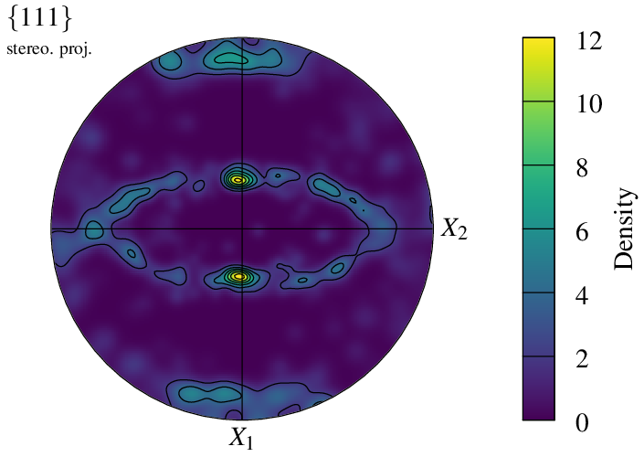
A density field is computed by assigning a kernel to each pole, which is defined by -pfkernel (default normal(theta=3)). A different value changes the intensity of the density field:
$ neper -V n200-psc.tess -space pf            \
           -pfmode density                    \
           -pfkernel "normal(theta=5)"        \
           -datacellscale 0:1:2:3:4:5:6       \
           -print img16
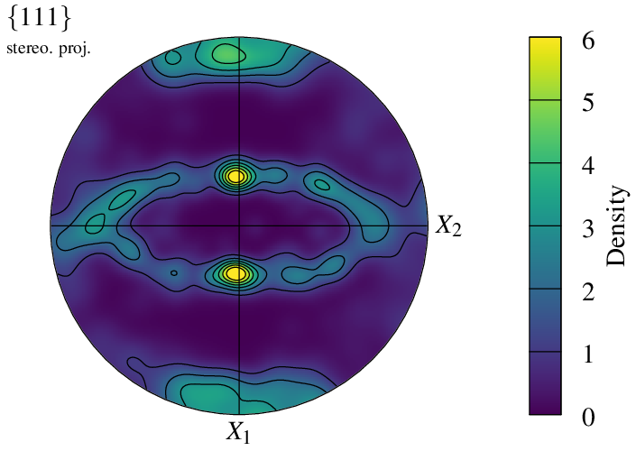
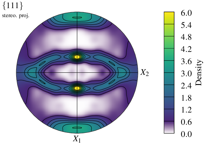
Symmetry conditions in the reference coordinate system can be defined using -pfsym (default monoclinic). It can be set to orthotropic:
$ neper -V n200-psc.tess -space pf            \
           -pfmode density                    \
           -pfkernel "normal(theta=5)"        \
           -pfsym orthotropic                 \
           -datacellscale 0:1:2:3:4:5:6       \
           -print img17
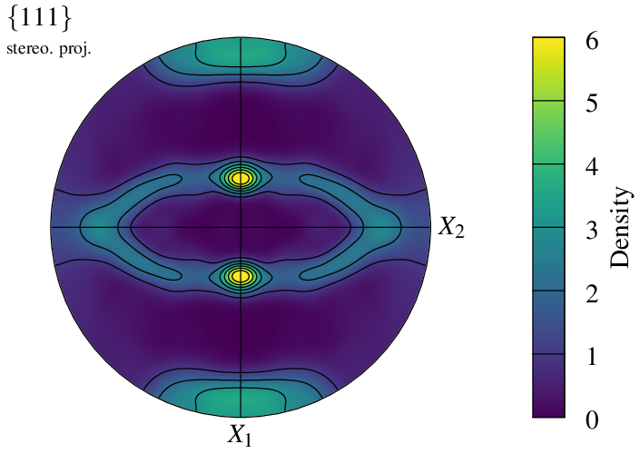
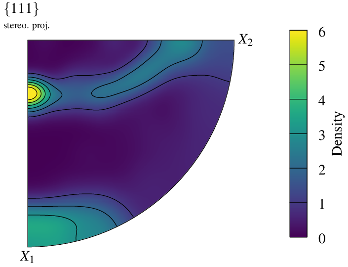
In the case of orthotropic symmetry, the pole figure can be reduced to one quarter using -pfsym quarter (default full):
$ neper -V n200-psc.tess -space pf            \
           -pfmode density                    \
           -pfkernel "normal(theta=5)"        \
           -pfsym orthotropic                 \
           -pfshape quarter                   \
           -datacellscale 0:1:2:3:4:5:6       \
           -print img18
The density field is defined on a regular grid, whose dimensions can be modified using -pfgridsize. While the default value of 200 provides a good balance between quality and computation time, the option can be used to speed up generation or, at the opposite, increase quality:
$ neper -V n200-psc.tess -space pf            \
           -pfmode density                    \
           -pfkernel "normal(theta=5)"        \
           -datacellscale 0:1:2:3:4:5:6       \
           -pfsym orthotropic                 \
           -pfgridsize 30                     \
           -print img19                       \
           -pfgridsize 300                    \
           -print img20


It is possible to specify which color scheme to use for the density plot, using -datacellcolscheme (see Color Maps for Real Values):
$ neper -V n200-psc.tess -space pf            \
           -pfmode density                    \
           -pfkernel "normal(theta=5)"        \
           -pfsym orthotropic                 \
           -datacellscale 0.0:6               \
           -datacellcolscheme "viridis:fade"  \
           -print img21
Working From an Orientation Input
A pole figure can be generated from an orientation file by loading it as a custom input (see Input Data). For instance, consider an orientation file, n100.ori, generated by Tessellation Module (-T):
$ neper -T -n 100 -for ori -o n100
The file can be loaded to the Visualization Module (-V) and plotted as a pole figure as follows:
$ neper -V n100.ori -space pf -print img22
Note
In -space pf, a custom input is interprated as an orientation file by default.
The command produces the same image as if the orientations were read from a tessellation with the same orientations.
Since the orientations are not attached to cells, they are no longer called cell but point (by default) in options -data* and -show*. For example, to specify symbol radii:
$ neper -V n100.ori -space pf -datapointrad 0.01+0.03*id/100 -print img23
Working From a Direction Input
A pole figure can be created from directions (instead of orientations) loaded as a custom input (see Input Data). For instance, consider file dir_file. The file can be loaded to the Visualization Module (-V), as a direction file, and plotted as a pole figure as follows:
$ neper -V "mydir(type=vector):file(dir_file)" -space pf -print img24
The data are not called point anymore but mydir (or any other name defining the custom input), which defines new options, -datamydir* and -showmydir.
$ neper -V "mydir(type=vector):file(dir_file)" -space pf \
        -datamydirrad 0.01+0.03*id/100                   \
        -print img25
Working From Multiple Inputs
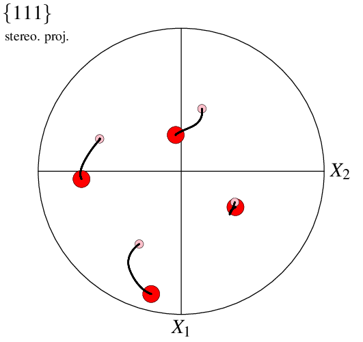
A pole figure can be created from multiple inputs loaded as custom inputs (see Input Data). This can, for example, be used to plot a (lattice) rotation path associated with plastic deformation. In the following, file ini contains an initial orientation, all its locations during plastic deformation, and fin the final orientation, all written as Rodrigues vectors.
Important
To plot lattice rotation paths, is it generally more efficient to use the method described in Plotting Orientation Trajectories instead of what is described here.
The initial orientation, rotation path and final orientation can be visualized as follows:
$ neper -V "final(type=ori):file(fin),initial(type=ori):file(ini),path(type=ori):file(all)" \
        -space pf                                     \
        -datainitialrad 0.030 -datainitialcol pink    \
        -datapathrad    0.005 -datapathcol    black   \
        -datafinalrad   0.060 -datafinalcol   red     \
        -print img26
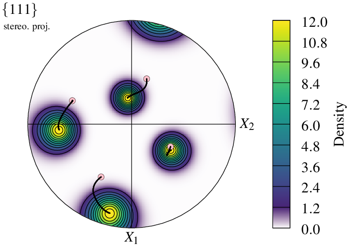
It is also possible to plot in density mode, in which case the mode applies only to the first input. This can be used, for example, to mimic an orientation spread at final state:
$ neper -V "final(type=ori):file(fin),initial(type=ori):file(ini),path(type=ori):file(all)" \
        -space pf                                     \
        -datainitialrad 0.030 -datainitialcol pink    \
        -datapathrad    0.005 -datapathcol    black   \
        -datafinalrad   0.000                         \
        -pfmode density,symbol                        \
        -datafinalscale 0.0:12                        \
        -datafinalcolscheme viridis:fade              \
        -pfgridsize 300 -pfkernel "normal(theta=8)"   \
        -print img27
Of course, it is also possible to represent final state using a file containing several orientations.