Plotting Orientation Trajectories

Important

Orientation trajectories described in a Simulation Directory (.sim) (whether they apply to (raster) tessellation cells or mesh elsets) can be plotted on a pole figure or an inverse pole figure, using the Visualization Module (-V) and its -space [i]pf options. This is done by plotting several simulation steps on the same figure, using -step.

Note

In principle, it is possible to plot orientation trajectories from a list of (unrelated) orientations loaded from a file; however, proper visualization generally requires the orientation history (through steps), hence the recommended use of a Simulation Directory (.sim).

In the following, the results of a small FEPX simulation is used (n20.sim.tgz, derived from this FEPX example), which corresponds to the deformation to 10% (engineering) tensile strain of a 20-grain polycrystal :

$ neper -S n20.sim

========================    N   e   p   e   r    =======================
Info   : A software package for polycrystal generation and meshing.
Info   : Version 4.5.1
Info   : Built with: gsl|muparser|opengjk|openmp|nlopt|libscotch (full)
Info   : Running on 8 threads.
Info   : <https://neper.info>
Info   : Copyright (C) 2003-2022, and GNU GPL'd, by Romain Quey.
Info   : Loading initialization file `/home/rquey/.neperrc'...
Info   : ---------------------------------------------------------------
Info   : MODULE  -S loaded with arguments:
Info   : [ini file] (none)
Info   : [com line] n20.sim
Info   : ---------------------------------------------------------------
Info   : Reading input data...
Info   :   - Reading arguments...
Info   :     > Input files: tess msh config
Info   :     > Node number      : 3606
Info   :     > Element number   : 2201
Info   :     > Elset number     : 20
Info   :     > Partition number : 2
Info   :     > Step number      : 10
Info   :     > Node results     : coo
Info   :     > Elt results      : ori
Info   :     > Elset results    : ori
Info   : Elapsed time: 0.001 secs.
========================================================================

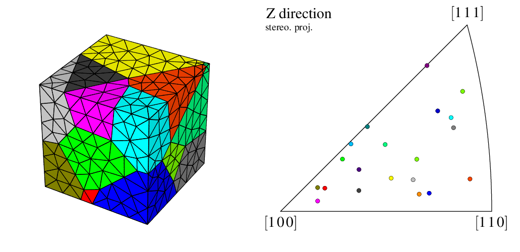
The polycrystal and its orientations on an IPF can be visualized as follows (the second command appends the two images to generate the image shown below):

$ neper -V n20.sim -imagesize 500:500 -cameraangle 15 -print img1 -space ipf -print img2
$ convert +append +repage -flatten img1.png img2.png img3.png

To reproduce exactly the images below, add the following line to your $HOME/.neperrc file (or to a local configuration file to be loaded with --rcfile):

neper -V -imagesize 500:500

Generalities

The orientation trajectories can be visualized by specifying several steps to -step. Using -step all, all steps are printed:

$ neper -V n20.sim -space ipf -step all -print img4

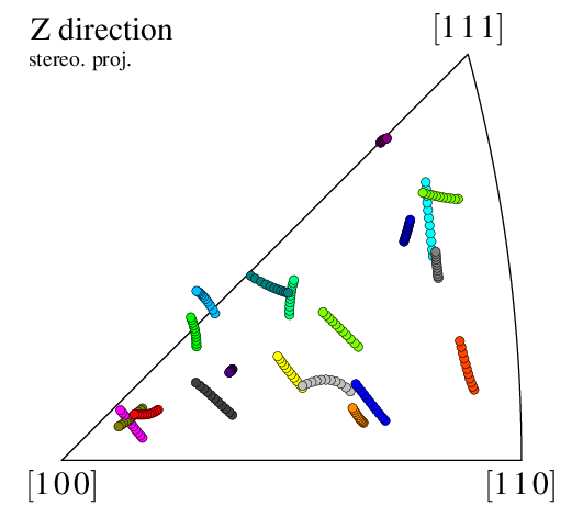
The orientations at successive steps are plotted on top of each other, using the same symbols.

Note

Orientation trajectories can go out of the standard triangle just as if the inverse pole figure was complete (not reduced to the standard triangle under crystal symmetry conditions).

Configuring the Symbol Plot

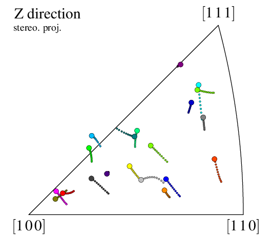
The way data are represented can be modified at large, as described in Plotting a Pole Figure (using elset instead of cell, since the results apply to a mesh). The step variable can also be used to plot orientations differently for each step. For example, to plot the last orientations using a larger symbol than the others (the “rotation path”):

$ neper -V n20.sim -space ipf -step all -dataelsetrad "real:((step<10)?0.008:0.024)" -print img5