Processing EBSD-type data
An experimental EBSD (orientation) map can be written as a Raster Tessellation File (.tesr) and visualized using the Visualization Module (-V). It can also be post-processed using the Simulation Module (-S), just as a mesh (and simulation results) can be.
Writing EBSD-type data as a Raster Tessellation File (.tesr)
An EBSD map typically consists of an orientation field described over a 2D grid. This can be described by a Raster Tessellation File (.tesr). An example of an EBSD map comprising \(3 \times 4\) pixels of size 0.001 is provided below (n2.tesr):
***tesr
 **format
   2.1
 **general
   2
   4 3
   0.001000000000 0.001000000000
 **oridata
   rodrigues:active
   ascii
   0.497071991874    0.751536029443   -0.324435016090
   0.450508625443    0.778380114981   -0.314292142975
  -2.500450755483    0.574774285761    2.818266339832
  -2.640295868326    0.613322889998    2.986906001722
   0.461530296952    0.723425478677   -0.335158513196
  -2.320688155349    0.549041867222    2.520971641905
  -2.355181399597    0.486342836815    2.739196570132
  -2.366437134562    0.745092186202    2.707700283931
  -2.680163356497    0.715754776276    3.187546229403
  -2.384540616434    0.667255925120    2.619216702767
  -2.694443582845    0.730843654602    2.969465573439
  -2.235296365544    0.532494712165    2.629239250625
***end
Note
See the description of a Raster Tessellation File (.tesr) for details on the structure. Voxel is used instead of pixel in the following, and in Neper in general.
The EBSD map can be visualized, colored by orientation, using the Visualization Module (-V):
$ neper -V n2.tesr -datavoxcol ori -print img1

Note
The orientation color key itself is not generated but can be obtained as detailed in Plotting an Orientation Color Key.
In the EBSD map, it may also occur that a voxel is not assigned any orientation. This can be indicated using the **oridef section:
***tesr
 **format
   2.1
 **general
   2
   4 3
   0.001000000000 0.001000000000
 **oridata
   rodrigues:active
   ascii
   0.497071991874    0.751536029443   -0.324435016090
   0.450508625443    0.778380114981   -0.314292142975
  -2.500450755483    0.574774285761    2.818266339832
  -2.640295868326    0.613322889998    2.986906001722
   0.461530296952    0.723425478677   -0.335158513196
  -2.320688155349    0.549041867222    2.520971641905
  -2.355181399597    0.486342836815    2.739196570132
  -2.366437134562    0.745092186202    2.707700283931
   0.000000000000    0.000000000000    0.000000000000
  -2.384540616434    0.667255925120    2.619216702767
  -2.694443582845    0.730843654602    2.969465573439
  -2.235296365544    0.532494712165    2.629239250625
 **oridef
   ascii
   1 1 1 1 1 1 1 1 0 1 1 1
***end
Note
Voxels for which the orientation is unknown (indicated 0 in the **oridef section) must still be assigned an orientation in the **oridata section, as a placeholder.
The EBSD map can be visualized as before:
$ neper -V n2b.tesr -datavoxcol ori -print img2

The “unindexed” voxels appear in gray by default, and their color can be changed using option -datavoxcol.
Finally, cells (or “grains”) can be defined using the **cell and **data sections:
***tesr
 **format
   2.1
 **general
   2
   4 3
   0.001000000000 0.001000000000
 **cell
   2
  *id
   1 2
 **data
   ascii
2 2 1 1 2 1 1 1 1 1 1 1
 **oridata
   rodrigues:active
   ascii
   0.497071991874    0.751536029443   -0.324435016090
   0.450508625443    0.778380114981   -0.314292142975
  -2.500450755483    0.574774285761    2.818266339832
  -2.640295868326    0.613322889998    2.986906001722
   0.461530296952    0.723425478677   -0.335158513196
  -2.320688155349    0.549041867222    2.520971641905
  -2.355181399597    0.486342836815    2.739196570132
  -2.366437134562    0.745092186202    2.707700283931
   0.000000000000    0.000000000000    0.000000000000
  -2.384540616434    0.667255925120    2.619216702767
  -2.694443582845    0.730843654602    2.969465573439
  -2.235296365544    0.532494712165    2.629239250625
 **oridef
   ascii
   1 1 1 1 1 1 1 1 0 1 1 1
***end
Note
The lines highlighted above indicate that there are 2 cells of numbers (or “ids”) 1 and 2. The *id section is optional if the cells are numbered contiguously from 1. The **data section should always contain numbers contiguously numbered from 1 (0 can be used to represent empty voxels), where 1 represents the first cell, 2 the second cell, etc. (independently of the cell ids provided in *id).
The EBSD map can be visualized, colored by its cell ids (which is the default), as follows:
$ neper -V n2c.tesr -print img3

Note
The **data, **oridata and **oridef sections are independent from each other, so that a cell may contain voxels that do not have any orientation, or a voxel that has an orientation may not belong to any cell.
Finally, it is a good idea to specify the crystal symmetry, using the *crysym section:
***tesr
 **format
   2.1
 **general
   2
   4 3
   0.001000000000 0.001000000000
 **cell
   2
  *id
   1 2
  *crysym
   cubic
 **data
   ascii
2 2 1 1 2 1 1 1 1 1 1 1
 **oridata
   rodrigues:active
   ascii
   0.497071991874    0.751536029443   -0.324435016090
   0.450508625443    0.778380114981   -0.314292142975
  -2.500450755483    0.574774285761    2.818266339832
  -2.640295868326    0.613322889998    2.986906001722
   0.461530296952    0.723425478677   -0.335158513196
  -2.320688155349    0.549041867222    2.520971641905
  -2.355181399597    0.486342836815    2.739196570132
  -2.366437134562    0.745092186202    2.707700283931
   0.000000000000    0.000000000000    0.000000000000
  -2.384540616434    0.667255925120    2.619216702767
  -2.694443582845    0.730843654602    2.969465573439
  -2.235296365544    0.532494712165    2.629239250625
 **oridef
   ascii
   1 1 1 1 1 1 1 1 0 1 1 1
***end
Processing the Data
A Raster Tessellation File (.tesr) (n2c.tesr) can be written as a Simulation Directory (.sim), for post-processing. This is simply done as follows:
$ neper -T -loadtesr n2d.tesr -for sim
The resulting simulation directory is simply structured as follows:
n2d.sim
└── inputs
    └── simulation.tesr
Cell properties can then be computed using option -rescell of the Simulation Module (-S), as follows:
$ neper -S n2d.sim -rescell ori
The resulting simulation directory is simply structured as follows:
n2d.sim
├── inputs
│   └── simulation.tesr
└── results
    └── cells
        └── ori
            └── ori.step0
Note
For consistency with actual simulation results, the result files are suffixed .step0, which denotes the initial state.
The map can then be colored following its average cell orientations (compare to the first image):
$ neper -V n2d.sim -datacellcol ori -print img4

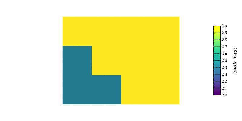
Cell properties, such as the “grain orientation spread”, gos, can be computed:
$ neper -S n2d.sim -rescell gos
The resulting simulation directory is simply structured as follows:
n2d.sim
├── inputs
│   └── simulation.tesr
└── results
    └── cells
        ├── gos
        │   └── gos.step0
        └── ori
            └── ori.step0
The data are simply formatted and can be accessed easily:
$ more n2d.sim/results/cells/gos/gos.step0
3.124415538011
2.405535676705
The map can then be colored following its cell gos values:
$ neper -V n2d.sim -datacellcol real:gos -datacellscale 2.0:3.0 -datacellscaletitle "GOS (degrees)" -print img5
$ convert img5.png img5-scale.png -gravity East -composite img5.png
This originally produces a PNG file named img5.png for the map and a PNG file named img5-scale.png for the scale bar, which is included to img5.png thanks to convert.