Using Neper from Python#
Note
This tutorial presents the Python Interface. Read first: Generating a Tessellation from Statistical Cell Properties (-T), Meshing a Tessellation (-T, -M) and Post-Processing and Visualizing Simulation Results (-S, -V).
The plots are made with Matplotlib. To reproduce exactly the images below, use the following settings (the Neper images are generated with imagesize="800:400"):
import numpy as np
import matplotlib.pyplot as plt
import neper

neper.set_defaults(rcfile="none")
plt.rcParams.update({"figure.figsize": (6, 3.6), "savefig.dpi": 100})
The Python Interface runs Neper’s modules from Python, reads their results into NumPy arrays, and passes NumPy arrays to Neper. This makes it possible to combine Neper with Python’s scientific libraries, e.g., to analyze tessellations, meshes and simulation results, plot them, carry out parametric studies, or visualize data computed in Python.
Analyzing the Cells of a Tessellation#
A tessellation with grain-growth properties (see Generating a Tessellation from Statistical Cell Properties (-T)) is generated with the cell equivalent diameters and sphericities as statistics:
res = neper.T(n=1000, morpho="diameq:lognormal(1,0.35),1-sphericity:lognormal(0.145,0.03)",
              statcell="diameq,sphericity")
The statistics are returned by res.stat("cell"), as a dictionary indexed by the keys of statcell. The equivalent diameters, normalized by their average (as in -morpho), are then compared to the prescribed lognormal distribution:
stat = res.stat("cell")
diameq = stat["diameq"] / stat["diameq"].mean()

d = np.linspace(0.01, 2.5, 200)
s2 = np.log(1 + 0.35**2)    # lognormal distribution of mean 1 and standard deviation 0.35
pdf = np.exp(-(np.log(d) + s2 / 2)**2 / (2 * s2)) / (d * np.sqrt(2 * np.pi * s2))

plt.hist(diameq, bins=30, density=True, label="tessellation")
plt.plot(d, pdf, label="prescribed")
plt.xlabel("normalized equivalent diameter")
plt.ylabel("probability density")
plt.legend()
plt.savefig("img1.png", bbox_inches="tight")
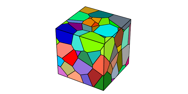
The standard deviation of diameq is 0.350, as prescribed.
Running a Parametric Study#
A Python loop runs Neper for different parameter values. For example, to generate tessellations of different cell size distributions and compute the actual standard deviations:
for sd in [0.1, 0.2, 0.35, 0.5]:
    res = neper.T(n=200, morpho=f"diameq:lognormal(1,{sd}),1-sphericity:lognormal(0.145,0.03)",
                  statcell="diameq", o=f"sd{sd}")
    diameq = res.stat("cell")["diameq"]
    print(f"{sd:.2f} {diameq.std() / diameq.mean():.3f}")
This prints:
0.10 0.101
0.20 0.200
0.35 0.348
0.50 0.478
Note
Since each run is a separate process, the runs can also be carried out in parallel, e.g. using concurrent.futures.ThreadPoolExecutor, with a reduced number of threads each (threads=...).
Processing Simulation Results#
The results of a small FEPX simulation are used (n20.sim.tgz, see Plotting Orientation Trajectories (-S, -V)), which corresponds to the deformation to 10% tensile strain along z of a 20-grain polycrystal. The node displacements are computed by the Simulation Module (-S) (which writes them in the simulation directory; you may want to work on a copy of it), and the simulation directory is read:
neper.S("n20.sim", resnode="disp")
sim = neper.read("n20.sim")
The strain is computed from the displacements of the nodes of the top domain face (whose initial height is 1):
disp = sim.read("nodes", "disp")                 # (steps, nodes, 3)
top = sim.mesh().nsets["z1"] - 1
strain = disp[:, top, 2].mean(axis=1)
The grain rotations are computed from the grain orientations, using neper.ori_angle and the orientation descriptor of the simulation, sim.orides (Rodrigues vectors):
ori = sim.read("elsets", "ori")                  # (steps, elsets, 3)
rotation = neper.ori_angle(ori, ori[0], sim.orides)

plt.plot(100 * strain, rotation, color="gray", lw=1)
plt.plot(100 * strain, rotation.mean(axis=1), color="black", lw=2, label="average")
plt.xlabel("strain (%)")
plt.ylabel("grain rotation (°)")
plt.legend()
plt.savefig("img2.png", bbox_inches="tight")
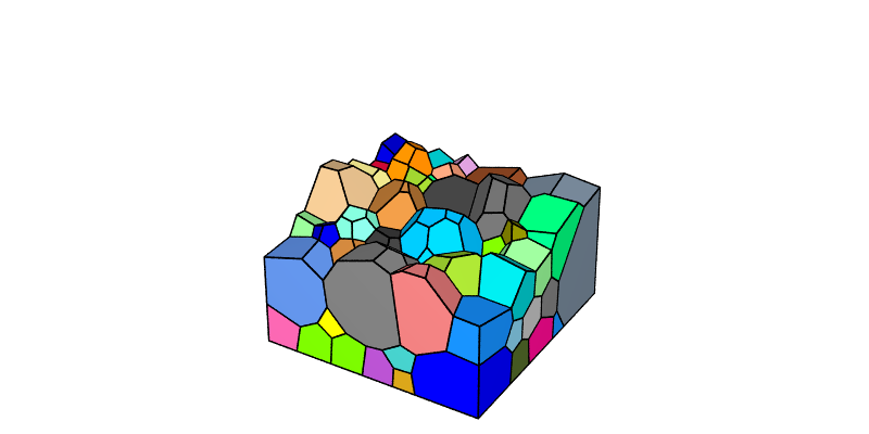
Finally, the grain rotations are written to the simulation directory, as a new result, which can then be used as any other result by the Simulation Module (-S) and the Visualization Module (-V):
sim.write("elsets", "rotation", rotation)
neper.V("n20.sim", step=10, imagesize="800:400", dataelsetcol="real:rotation",
        dataelsetscale="0:6", print="img3")
